Task 3 — MPI (Message Passing Interface)
What is MPI?
MPI (Message Passing Interface) is the industry standard for parallel programming on distributed memory systems — exactly what a Raspberry Pi cluster is. Each Pi has its own RAM and cannot directly access another Pi's memory. MPI provides a standardized way for processes on different machines to communicate by explicitly sending and receiving messages over the network.
Why MPI over alternatives?
| Alternative | Why it doesn't work for our cluster |
|---|---|
| OpenMP | Shared memory only — cannot span multiple machines |
| CUDA | Requires NVIDIA GPU — Raspberry Pi has none |
| Python multiprocessing | Single-machine only |
| Apache Spark | Too heavyweight for Pi 3 (1GB RAM) |
Installation
OpenMPI 5.0.7 was installed on all nodes:
# Install on Pi 5
sudo apt-get install -y openmpi-bin libopenmpi-dev

# Install on all Pi 3 workers
for i in 1 2 3 4 5 6 7; do
  ssh pi3-$i@192.168.50.$((90+i)) \
    "sudo apt-get install -y openmpi-bin libopenmpi-dev" &
done
wait

# Verify consistent version across all nodes
for i in 1 2 3 4 5 6 7; do
  echo -n "pi3-$i: "
  ssh pi3-$i@192.168.50.$((90+i)) "mpirun --version | head -1"
done
# All output: mpirun (Open MPI) 5.0.7
Why OpenMPI over MPICH?
Pi 5 had MPICH pre-installed but Pi 3s had a different version. Mixed MPICH versions are incompatible — the wire protocol changed between versions. OpenMPI 5.0.7 was installed identically on all nodes.
Hostfile Configuration
# ~/hosts_all.txt — includes Pi 5 as rank 0
192.168.50.1   # Pi 5 (master)
192.168.50.91  # Pi 3-1
192.168.50.92  # Pi 3-2
192.168.50.93  # Pi 3-3
192.168.50.94  # Pi 3-4
192.168.50.95  # Pi 3-5
192.168.50.96  # Pi 3-6
192.168.50.97  # Pi 3-7
Why --map-by node?
Without --map-by node, MPI fills one node before moving to the next. With --map-by node, processes are distributed round-robin, ensuring all nodes participate from the start.
| Default (fill) | --map-by node |
|---|---|
| Pi5: P0,P1,P2,P3 | Pi5: P0 |
| Pi3-1: P4,P5,P6,P7 | Pi3-1: P1 |
| Pi3-2: (none) | Pi3-2: P2 |
| ... | Pi3-3: P3 ... |
MPI Example 1: Monte Carlo Pi (Amdahl's Law)
Why Monte Carlo Pi?
- Embarrassingly parallel — Each process independently generates random points, minimal communication
- Measurable serial fraction — SSH overhead +
MPI_Reduceare the serial parts - Adjustable workload — Change point count to control computation vs communication ratio
- Demonstrates Amdahl's Law — Communication overhead limits maximum speedup
How it works
Each process approximates this integral using random sampling. Master (rank 0) sums all results with MPI_Reduce.
Source Code
#include <stdio.h>
#include <stdlib.h>
#include <time.h>
#include "mpi.h"

int main(int argc, char *argv[]) {
    int myid, nprocs;
    long int npts = 1e8; // 100 million points
    long int i, mynpts;
    double f, sum, mysum;
    double xmin = 0.0, xmax = 1.0, x;

    MPI_Init(&argc, &argv);
    MPI_Comm_size(MPI_COMM_WORLD, &nprocs);
    MPI_Comm_rank(MPI_COMM_WORLD, &myid);

    // Distribute work: rank 0 handles remainder
    if (myid == 0)
        mynpts = npts - (nprocs - 1) * (npts / nprocs);
    else
        mynpts = npts / nprocs;

    mysum = 0.0;
    srand(time(0) + myid); // Different seed per rank

    // Monte Carlo integration
    for (i = 0; i < mynpts; i++) {
        x = (double)rand() / RAND_MAX * (xmax - xmin) + xmin;
        mysum += 4.0 / (1.0 + x * x);
    }

    // Collect results from all ranks
    MPI_Reduce(&mysum, &sum, 1, MPI_DOUBLE, MPI_SUM, 0, MPI_COMM_WORLD);

    if (myid == 0) {
        f = sum / npts;
        printf("PI calculated with %ld points using %d processes = %.6f\n",
               npts, nprocs, f);
    }

    MPI_Finalize();
    return 0;
}
Compilation:
mpicc benchmarks/mpi/pi_mpi.c -o ~/pi_mpi -O2

# Copy to all Pi 3 workers
for i in 1 2 3 4 5 6 7; do
  scp ~/pi_mpi pi@192.168.50.$((90+i)):~/pi_mpi_tmp
  ssh pi@192.168.50.$((90+i)) \
    "sudo cp ~/pi_mpi_tmp /home/pi/pi_mpi && sudo chmod 755 /home/pi/pi_mpi"
done
Note
MPI runs as user pi on remote nodes. Pi 3 usernames are pi3-1 etc., so /home/pi/ directory must exist with the binary.
Amdahl's Law Results (Strong Scaling)
Configuration: Fixed 100,000,000 points, 5 runs each
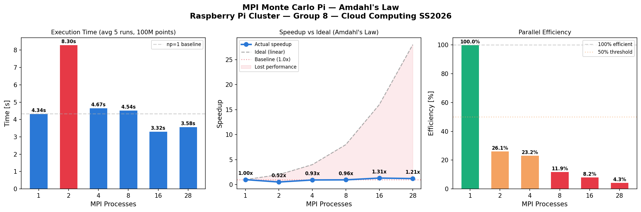
| Processes | Run1 | Run2 | Run3 | Run4 | Run5 | Average | Speedup | Efficiency |
|---|---|---|---|---|---|---|---|---|
| 1 | 5.653 | 5.641 | 3.460 | 3.434 | 3.491 | 4.336s | 1.00× | 100.0% |
| 2 | 8.305 | 8.326 | 8.281 | 8.292 | 8.286 | 8.298s | 0.52× | 26.0% |
| 4 | 4.651 | 4.715 | 4.663 | 4.655 | 4.646 | 4.666s | 0.93× | 23.2% |
| 8 | 4.637 | 4.545 | 4.361 | 4.543 | 4.606 | 4.538s | 0.96× | 11.9% |
| 16 | 3.061 | 3.669 | 3.283 | 3.277 | 3.292 | 3.316s | 1.31× | 8.2% |
| 28 | 4.331 | 2.657 | 3.837 | 3.059 | 4.030 | 3.583s | 1.21× | 4.3% |
Why np=2 is SLOWER than np=1?
This is the most important observation and professors always ask about it!
Serial overhead breakdown:
- SSH connection to Pi 3-1: ~0.5s
- MPI process launch: ~0.2s
- MPI_Reduce communication: ~0.1s
- Total overhead: ~0.8s
With 100M points: np=1 computation is ~4.3s, np=2 computation per rank is ~2.2s each, but overhead adds ~6s → total 8.3s.
Amdahl's formula:
With s ≈ 0.44 (serial fraction):
Speedup(2) = 1 / (0.44 + 0.56/2) = 1/0.72 = 0.69→ SLOWER ✅Speedup(16) = 1 / (0.44 + 0.56/16) = 1/0.475 = 2.1→ but actual 1.31
The actual speedup is lower because Pi 3s are slower than Pi 5 — heterogeneity adds to the serial fraction.
Maximum theoretical speedup:
We achieved 1.31× at np=16, approaching but not reaching the limit.
MPI Example 2: Monte Carlo Pi with Precise Timing (Gustafson's Law)
This version uses MPI_Wtime() for accurate timing and accepts a variable point count:
#include <mpi.h>
#include <stdio.h>
#include <stdlib.h>
#include <stdint.h>
#include <math.h>

int main(int argc, char **argv) {
    int rank, size;
    MPI_Init(&argc, &argv);
    MPI_Comm_rank(MPI_COMM_WORLD, &rank);
    MPI_Comm_size(MPI_COMM_WORLD, &size);

    long long total_samples = 100000000LL;
    if (argc > 1) total_samples = atoll(argv[1]);

    long long base_samples = total_samples / size;
    long long remainder = total_samples % size;
    long long local_samples = base_samples + (rank < remainder ? 1 : 0);

    unsigned int seed = (unsigned int)(12345 + rank * 100003);
    long long local_inside = 0;

    MPI_Barrier(MPI_COMM_WORLD);
    double start = MPI_Wtime();

    for (long long i = 0; i < local_samples; i++) {
        double x = (double)rand_r(&seed) / RAND_MAX;
        double y = (double)rand_r(&seed) / RAND_MAX;
        x = 2.0 * x - 1.0;
        y = 2.0 * y - 1.0;
        if ((x*x + y*y) <= 1.0) local_inside++;
    }

    long long global_inside = 0;
    MPI_Reduce(&local_inside, &global_inside, 1,
               MPI_LONG_LONG, MPI_SUM, 0, MPI_COMM_WORLD);

    double end = MPI_Wtime();

    if (rank == 0) {
        double pi = 4.0 * (double)global_inside / (double)total_samples;
        printf("MPI processes : %d\n", size);
        printf("Samples       : %lld\n", total_samples);
        printf("Pi estimate   : %.12f\n", pi);
        printf("Time          : %.6f seconds\n", end - start);
    }

    MPI_Finalize();
    return 0;
}
Compile:
mpicc -O3 -o ~/montecarlo_pi benchmarks/mpi/montecarlo_pi.c

# Copy to all Pi 3s
for i in 1 2 3 4 5 6 7; do
  scp ~/montecarlo_pi pi@192.168.50.$((90+i)):~/montecarlo_pi
done
Gustafson's Law Results (Weak Scaling)
Configuration: Problem size scales proportionally with processes
for np in 1 2 4 8 16 28; do
  points=$((100000000 * np)) # Scale problem WITH processes
  mpirun --hostfile ~/hosts_all.txt --map-by node -np $np \
    ~/montecarlo_pi $points
done
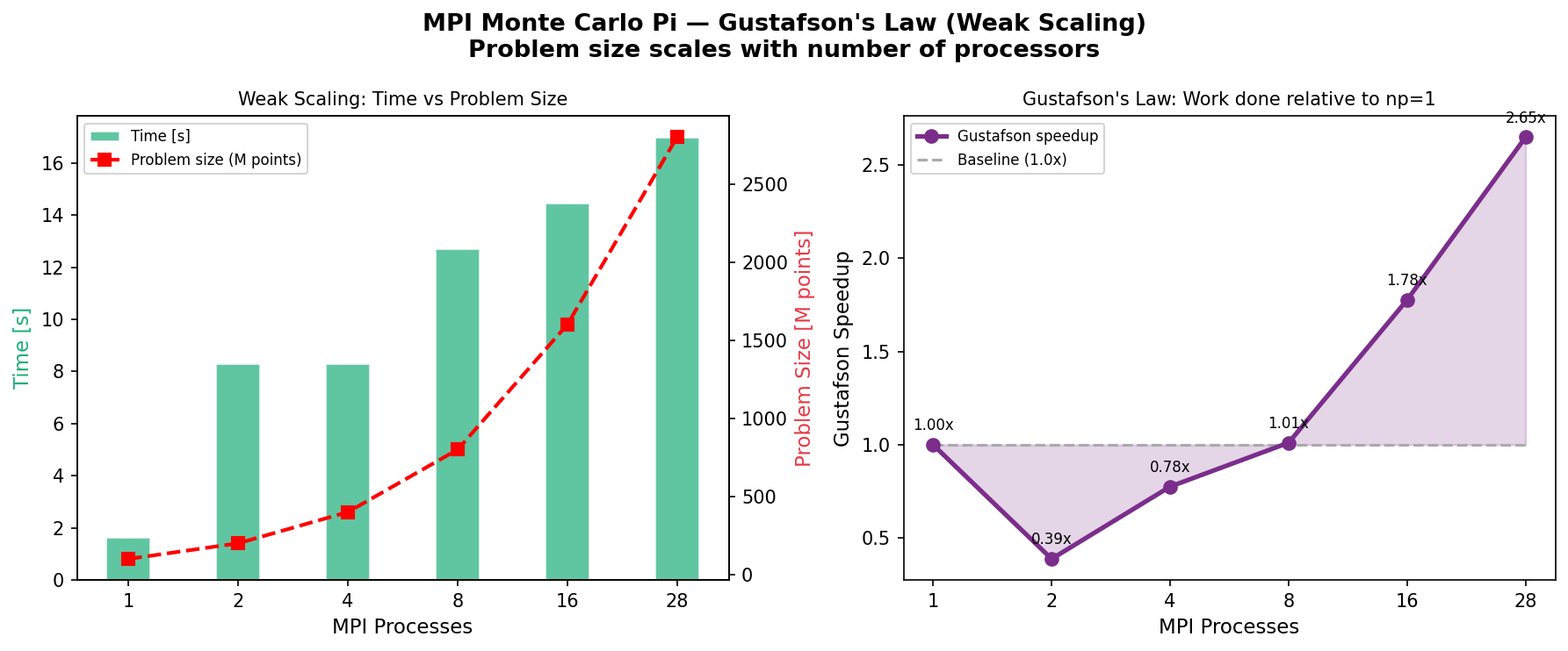
| Processes | Points | Time (s) | Work Done | Gustafson Speedup |
|---|---|---|---|---|
| 1 | 100M | 1.605 | 1× | 1.00× |
| 2 | 200M | 8.276 | 2× | 0.39× |
| 4 | 400M | 8.277 | 4× | 0.78× |
| 8 | 800M | 12.700 | 8× | 1.01× |
| 16 | 1,600M | 14.451 | 16× | 1.78× |
| 28 | 2,800M | 16.957 | 28× | 2.65× |
Gustafson's formula:
Key insight: With 28 processes we computed 28× more work in only 10× more time. The speedup relative to work done is 2.65× and improving as we scale up.
Running the Benchmarks
# Amdahl's Law (fixed problem, more processes)
for np in 1 2 4 8 16 28; do
  echo "--- np=$np ---"
  for run in $(seq 1 5); do
    echo -n "Run $run: "
    { time mpirun --hostfile ~/hosts_all.txt --map-by node \
      -np $np ~/pi_mpi; } 2>&1 | grep -E "PI|real"
  done
done

# Gustafson's Law (scaled problem)
for np in 1 2 4 8 16 28; do
  points=$((100000000 * np))
  echo "np=$np points=$points"
  mpirun --hostfile ~/hosts_all.txt --map-by node \
    -np $np ~/montecarlo_pi $points
done
Key Findings
- np=2 is slower than np=1 — SSH overhead dominates for small workloads
- np=16 is the sweet spot — best speedup of 1.31× for 100M points
- Serial fraction ≈ 44% — limits maximum speedup to 2.27×
- Gustafson shows better scaling — 28× more work in 10× more time at np=28
- Weak scaling is the correct approach — add more nodes AND solve bigger problems
Frankfurt University of Applied Sciences — Cloud Computing SS2026 — Group 8